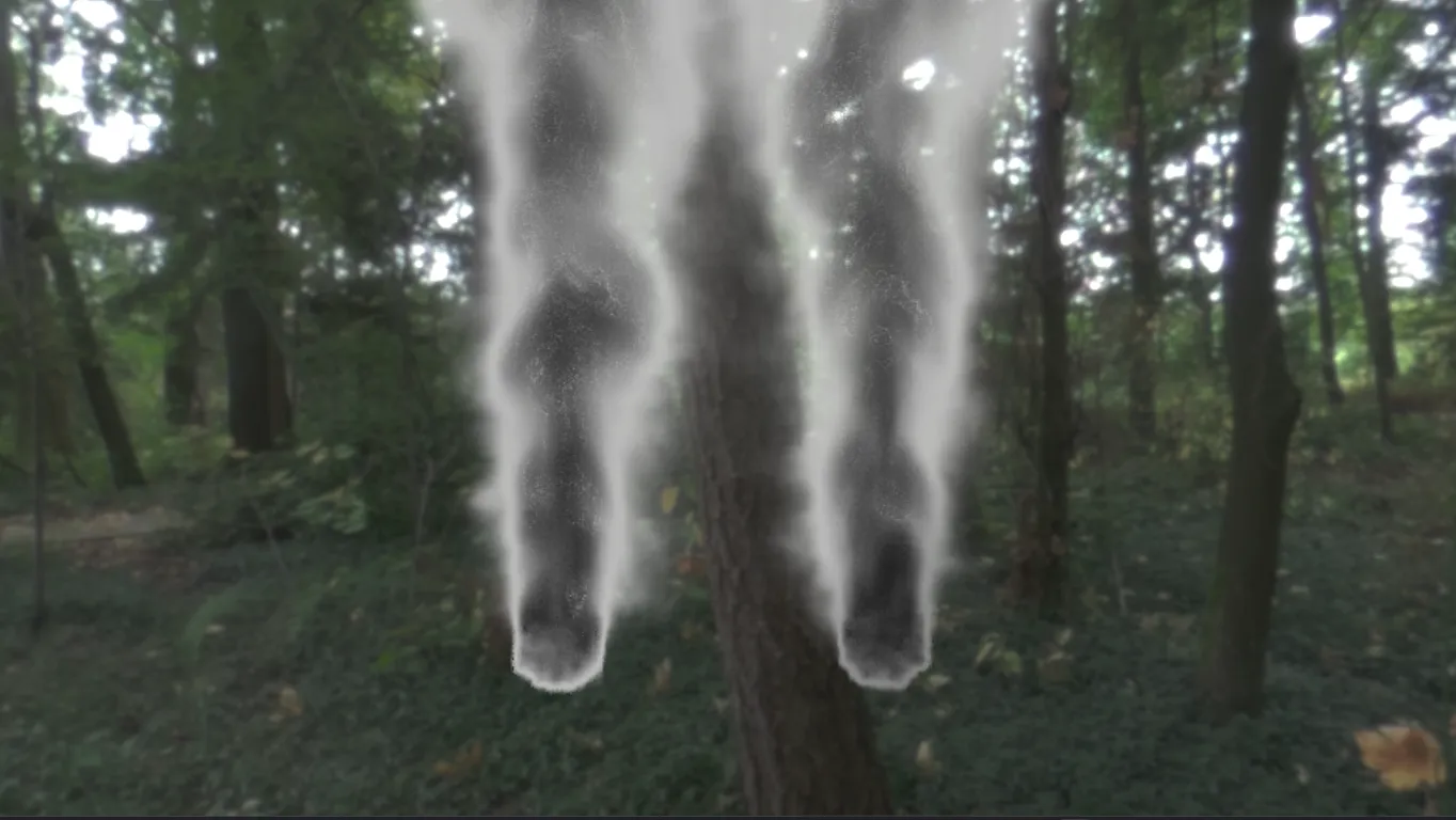
Smoke Simulation

Introduction

After seeing the Coding Adventures series by Sebastian Lague on fluid simulation and smoke simulation ¹ I was inspired to experiment with this myself. Initially I wanted to make a particle-based fluid simulator, but because that is rarely used in real-time applications I later settled on making a 3D Eularian smoke simulator. I achieved this by implementing a MAC grid system with a Jacoby pressure solver. The rendering is achieved using a raymarching algorithm that works in the same voxel grid as the pressure solver.

This post is aimed towards people with at minimum a basic game development aspiration and some basic math knowledge or at least the ability to read mathematical equations.

All interactive elements on this page are inspired by the wonderful visualisations from Sebastian Lague. The web dev part is made with help from Claude, since my web development skills are not great at the time of writing. I recommend to read this on desktop to fully profit from the interactive elements.

Notation

This section is meant to clarify or explain certain mathematical notations. If you are familiar with them, feel free to skip this part.

I take as any arbitrary value. This means that any function using this is applicable for multiple parameters.

means that the number is a positive integer.

denotes the length of vector

is the partial derivative with respect to . This can be seen as “the rate of change on the axis” or in some cases “the difference in the axis” (mostly used for velocities). For example for the velocity, it can be written out in code as

float ddx = MAC::VelocityXBuffer[center + int3(1,0,0)] - MAC::VelocityXBuffer[center]

denotes the gradient. In 3D, this is .

Simulation

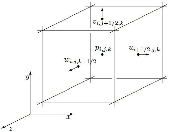
Grid

At the core of the simulation lies a MAC grid storage system. A MAC grid is a kind of voxel grid storage technique where different values are stored at different positions in the grid. In my case, the grid has the pressures, cell types, temperature and concentration stored at the center of each cell, whereas the velocities are stored on the face centers of the cells. This means that the dimensions of the pressure and type buffers need to be where . The velocity component buffers need to have one extra entry in their respective axis to ensure all sides have values. I will follow the convention that any parameter at the center of cell in the grid can be written as .

The algorithm

All fluid simulations run on the Navier Stokes equation ³

where is the velocity, is the pressure, is the fluid density and are any applicable external forces.
Since smoke has zero viscosity, can be removed from the equation.
For the code, I will use the convention that the velocities stored at a position are of the lesser side. So, is stored at u[i][j][k], etc.

With this equation, all passes can be broken down and this can be calculated piecewise, for which I have chosen to make one compute shader per pass.

I made use of Texture3D objects in HLSL to store the buffers. This because I can then easily index it using a uint3 and offload the trilinear sampling needed in the advection pass to the GPU’s built-in sampling functions.

Pressure

Rearranging the Navier Stokes equation gives the following formula¹ for pressure at a point in the grid

where is the time-step since the last simulation frame. For any cell that is solid the pressure and velocity can be set to 0.

This equation is not enough on its own, since there need to be proper bounding conditions to ensure the pressure is calculated correctly. For this, I am using the slip condition which says that for all the solid boundaries, the pressure difference is zero, ensuring that the smoke can easily slip along the boundary. This also means that the edge velocities will always be zero.

Applying this formula on a MAC grid is not enough, because as you might have already spotted the cells are dependent on each other. This means that there needs to be an algorithm in place to relax the values to near their equilibrium. A simple way to do this is the “Just running the shader a lot of times” method or more formerly known as the Jacobi method. As you can probably also see from the visualisation, the pressure needs quite a lot of iterations to settle down. To get the most precise result you’d have to run the solver a large number of times, so to keep the system real-time for each pass of the solver the pressure is only updated a fixed amount of times (in my case 16).
To make this as performant as possible however, the best option is to utilise the GPU for this, but this poses the problem of race conditions, hence the need for the shader to use what’s called Red-Black computation. This algorithm first computes the values for the even cells and then for the odd cells. This works flawlessly, since the formula for pressure shows that no diagonal neighbours are being sampled.

Velocity

This is where the magic of the MAC grid comes to light. Since I have the pressure of all cell centers, getting the velocity is simply applying the pressure difference to alter the velocities. Written out for all axes:

Applying this pass satisfies the requirement that

or in other words that there is an equal amount of velocity leaving the cell as there is velocity entering.

In the visualisation, you’ll notice that not all pressures drop to zero as you would expect (because velocity tries to equalise the pressure difference). This is because the pressure solver cannot be run enough times to make for an absolute equilibrium.

What you can also notice from the simulation is that there forms a natural vortex pattern in the velocities. This effect will cause the smoke to spread out and create the mushroom cloud shape that is usually associated with rising smoke.

Advection

To make the velocities move through the volume the logical approach is to take the current velocity at one of the faces and move that velocity one time step forward.

where is any arbitrary value that needs to be advected and is its position.

This brings one major problem, namely that it is possible but very computationally difficult to distribute the velocity along all edges in the cell the velocity lands in. However, since this a sequence, the algorithm can instead move one step backwards and put that velocity at the position on the chosen face

This is computationally very simple, since that only takes two samples of the velocity texture(s). With this method, the second sample only needs to be the component of the face that is being computed.

Temperature and concentration

Specifically for smoke temperature and concentration are needed to make it act properly. Both of the variables are stored at the center of a cell and are advected the same way as the velocity. Spawners inject concentration into the grid, whereafter the buoyancy force ² is applied to the velocities to produce the initial velocity.

where and are non-zero constants that you can set to your liking, and .

This mutual dependency makes sure that velocities are calculated around the concentration field to make sure that the advection can function properly.

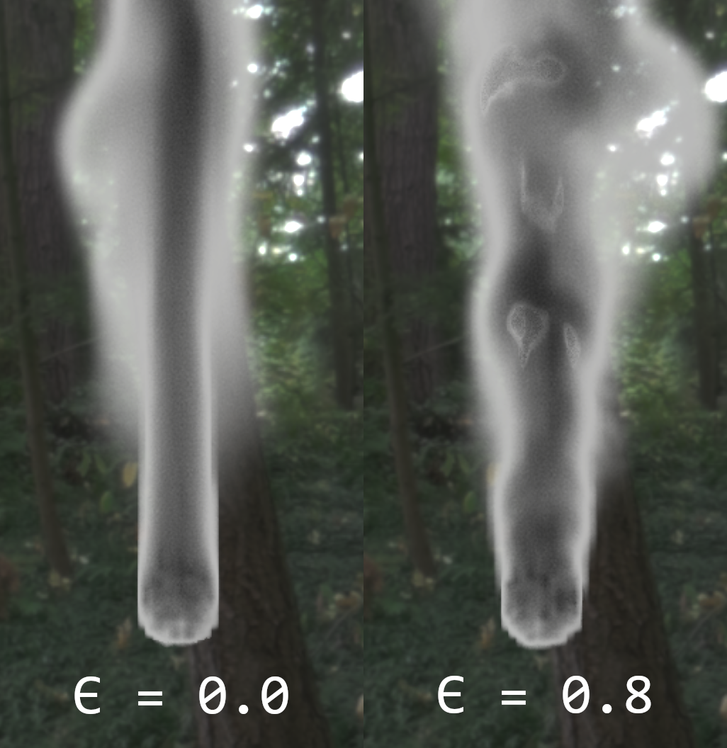
Vorticity

To accentuate the curliness of the smoke, vorticity can be applied⁴. This force tries to spin the smoke in a certain direction. It is calculated by first taking the angular velocity

whereafter that can be used to calculate the normalised vorticity location vector:

This vector can then be used to get the force that the vorticity is applying to the velocity field by crossing the location vector with the vorticity vector:

where controls how strong the effect of the vorticity is.

Rendering

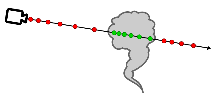
Rendering the smoke is done through a simple raymarching algorithm. In my implementation, the origin of the rays are snapped to the bounds of the fluid to not have to trace through a guaranteed empty space.

Each step of the raymarcher, the checked point is shifted over some step size ⁶. To make the trace more optimal, I make use of variable step sizes, since the precision needed decreases when either further away from the camera or deeper in the volume. Every time the trace switches state (inside or outside) the step sizes are reset to make the edges of the smoke look good.

Then I sample the concentration buffer to know how much if any smoke is at that point. All the concentration values are summed up, whereafter it is used to determine the final opacity and color of the pixel using the formula ⁷:

where is the total acquired concentration, is the absorbance coefficient, is the angle between the ray direction and the sunlight direction and is the eccentricity that defaults to 0.2.

This equation is made up of the three following effects:

• Beer’s law (green): Makes the smoke color darker the more concentration is captured in the raymarching.
• In-scattering (blue): Gives the smoke dark edges.
• Henyey-Greenstein Phase Function (orange): Adds silver-lining to the smoke, giving it brighter edges.

To make the smoke look more ‘smoke-like’ I apply the noise functions proposed in the talk ⁶. For this, I take their 3D noise texture and sample it with the algorithm present in the sample’s code.

Performance

With a reasonable 128x128x128 MAC grid system and 16 iterations of the pressure solver my simulation settled on an execution time of 13.52ms. This amounts to 13.00ms of the MAC solver and 0.52ms of the raymarcher. Because of the fact that this is too slow to embed in a render pass, I suggest that you run this at a resolution of 128x128x128 if you’re getting comparable results.

During the project, I have made several significant optimisations to my fluid solver and rendering algorithm. These include:

• More efficient use of GPU data types. These choices include using half over float or using Texture3D over a StructuredBuffer or ByteAddressBuffer.
• Making use of caching. This is very effective in the fluid solver because of the large amount of times a certain pixel is sampled. For example, the part of the pressure equation that involves velocity (negative divergence) can easily be cached since it stays constant throughout the iterations, removing the need to calculate that each iteration of the solver.
• Choosing the correct buffer type to minimise VRAM throughput.
• Utilising the GPU optimally. In my raymarcher, it is significantly better to do the steps on the GPU instead of one dispatch per step. This also optimises away some buffers that were needed.
• A thing that ⁶ proposed is to take variable steps through the volume. This does mean that the initial values and step increments need to be chosen correctly. In the case of my smoke sim there needs to be proper handling of when the ray is near the edges of the bounds, since this can create precision artifacts when rendering.
• If viable for looks implementations can render the smoke at half resolution and upscale later. This should give a 4x increase in performance.

Below is a table with the results of the optimisations listed above. Note that the measurements are done at different times into the development and might not resemble the final performance. Do however take these as a reference on how certain changes might impact performance.

Addition/Change	From	To	Relative
[Solver] Baseline	12.42ms	N/A	N/A
[Solver] Buffer ⟶ Texture	12.42ms	11.13ms	-10.4%
[Solver] Negative Divergence caching	20.05ms	13.16ms	-34.4%
[Solver] TypeBuffer to R8_UINT	13.16ms	12.91ms	-1.9%
[Marcher] Baseline	17.04ms	N/A	N/A
[Marcher] Steps on the GPU	14.80ms	8.71ms	-41.1%
[Marcher] Variable step size	7.78ms	3.04ms	-60.9%
[Marcher] Half resolution	3.04ms	0.78ms	-74.3%

Conclusion and Future Work

All in all this project taught me plenty of things about how to do things properly on the GPU. I did not manage to do everything that I wanted, since in the eight weeks I had for the project I spent a vast majority of the time with a broken advection algorithm. Even though this lost me a lot of time, the result still results in this blog post that I hope serves well as a reference for making your own smoke/fluid simulation. During the project I also looked way differently at smoke since now I know what forces make up the movements of smoke.

In the future, I am planning to maybe add light tracing in the mix as well as adding emittance based on temperature. This can then be expanded with ember particles to make for a nice pyrotechnics simulator.

I also do believe that a lot more performance can be squished out of the simulation with the right knowledge and tools. Sadly I did not have time to dive into the nitty-gritty details of my code.

References

Footnotes

1. S. Lague, “Coding Adventure: Simulating Smoke”, 2025, https://www.youtube.com/watch?v=Q78wvrQ9xsU ↩ ↩²

2. R. Bridson, “Fluid Simulation for Computer Graphics (Second Edition)”, 2016 ↩ ↩²

3. K. Crane, I. Llamas, S. Tariq, “Real-Time Simulation and Rendering of 3D Fluids (GPU Gems chapter 30)”, 2008, https://www.cs.cmu.edu/~kmcrane/Projects/GPUFluid/paper.pdf ↩

4. R. Fedkiw, J. Stam, H.W. Jensen, “Visual simulation of smoke”, 2001, https://dl.acm.org/doi/pdf/10.1145/383259.383260 ↩

5. R. Brucks, “Creating a Volumetric Ray Marcher”, 2016, https://shaderbits.com/blog/creating-volumetric-ray-marcher ↩

6. A. Schneider, ”: Methods (and madness) to model and render immersive real-time voxel-based clouds.”, 2023, https://d3d3g8mu99pzk9.cloudfront.net/AndrewSchneider/Nubis%20Cubed.pdf ↩ ↩² ↩³

7. E. Ge, D. Liang, Z. Zhang, “Fire Simulation and Rendering”, 2020, https://cs184-firesim.github.io/final-report/ ↩